Model Evaluation and Validation

• ID: ADS-L09
• Type: Model evaluation
• Audience: Intermediate
• Theme: Performance estimates must reflect how a model will be used

Learning objectives

By the end of this chapter, you should be able to:

• distinguish model evaluation from model validation;
• assign clear roles to training, validation, and test data;
• construct leakage-safe preprocessing and modelling pipelines;
• select metrics that match the prediction task and decision context;
• use cross-validation to estimate performance variability;
• tune a classification threshold without contaminating the test set;
• assess discrimination, calibration, subgroup performance, and uncertainty; and
• communicate model performance without overstating generalizability.

Why evaluation is more than reporting a score

A model can fit the available data well and still fail on new cases. Model evaluation asks how well a fitted model performs under a specified metric. Model validation asks whether that estimate remains credible for the intended population, time period, setting, and workflow.

The goal is therefore not to find the largest score. It is to obtain an honest estimate of future performance and understand where that estimate may fail.

A performance estimate is meaningful only when the data split, preprocessing, metric, threshold, and intended use are clearly defined.

A validation strategy starts with the deployment scenario

Before splitting data, identify what the model will encounter in practice. Random splitting is appropriate only when future observations are plausibly exchangeable with current observations.

Intended use	Preferred validation design	Main risk addressed
New independent observations from the same population	Stratified random split or stratified cross-validation	Class imbalance and sampling variation
Future observations	Forward or rolling time split	Temporal leakage and changing data distributions
New patients, customers, sites, or devices	Group-aware split	The same entity appearing in training and validation data
A new hospital, region, laboratory, or organization	Leave-one-group/site-out validation	Poor transportability across settings
Final confirmation after model development	Untouched holdout or external dataset	Optimism caused by repeated model selection

If observations are clustered, repeated, spatially related, or ordered in time, the split must preserve that structure.

Training, validation, and test data

The three partitions have different purposes:

• Training data estimate model parameters.
• Validation data guide model and hyperparameter choices.
• Test data provide one final estimate after all choices are fixed.

When the dataset is too small for a separate validation set, cross-validation can be performed within the training data. The test set must remain untouched.

from sklearn.model_selection import train_test_split

X_train, X_test, y_train, y_test = train_test_split(
    X,
    y,
    test_size=0.20,
    stratify=y,
    random_state=42,
)

stratify=y approximately preserves the class proportions. It does not solve group dependence, temporal structure, or distribution shift.

Prevent data leakage with pipelines

Data leakage occurs when information unavailable at prediction time influences model development. Common examples include:

• scaling or imputing before the split;
• selecting features using the complete dataset;
• creating predictors from future information;
• allowing repeated records from one entity into different folds; and
• tuning hyperparameters or thresholds on the test set.

Preprocessing should be fitted separately inside every training fold. A scikit-learn pipeline enforces this ordering.

from sklearn.compose import ColumnTransformer
from sklearn.impute import SimpleImputer
from sklearn.linear_model import LogisticRegression
from sklearn.pipeline import Pipeline
from sklearn.preprocessing import OneHotEncoder, StandardScaler

numeric_pipeline = Pipeline(
    steps=[
        ("imputer", SimpleImputer(strategy="median")),
        ("scaler", StandardScaler()),
    ]
)

categorical_pipeline = Pipeline(
    steps=[
        ("imputer", SimpleImputer(strategy="most_frequent")),
        ("encoder", OneHotEncoder(handle_unknown="ignore")),
    ]
)

preprocessor = ColumnTransformer(
    transformers=[
        ("numeric", numeric_pipeline, numeric_features),
        ("categorical", categorical_pipeline, categorical_features),
    ]
)

model = Pipeline(
    steps=[
        ("preprocess", preprocessor),
        ("classifier", LogisticRegression(max_iter=2_000)),
    ]
)

Cross-validation estimates variability

In k-fold cross-validation, the training data are divided into k folds. The model trains on k - 1 folds and is evaluated on the remaining fold, repeating until every fold has served as validation data.

from sklearn.model_selection import StratifiedKFold, cross_validate

cv = StratifiedKFold(n_splits=5, shuffle=True, random_state=42)

scores = cross_validate(
    model,
    X_train,
    y_train,
    cv=cv,
    scoring={
        "roc_auc": "roc_auc",
        "average_precision": "average_precision",
        "neg_log_loss": "neg_log_loss",
    },
    n_jobs=-1,
)

Report the fold-level distribution or a summary such as the mean and standard deviation. A mean alone hides instability.

import pandas as pd

cv_results = pd.DataFrame(scores)
summary = cv_results.filter(like="test_").agg(["mean", "std"]).T
print(summary)

When both hyperparameter tuning and an unbiased internal performance estimate are required, use nested cross-validation: an inner loop selects settings, and an outer loop estimates performance. For grouped or temporal data, replace the generic splitter with an appropriate group-aware or time-aware strategy.

Choose metrics from the consequence of error

Classification metrics

Let true positives be TP, false positives FP, true negatives TN, and false negatives FN.

Metric	Question answered	Important caution
Accuracy	What proportion of predictions is correct?	Can be misleading with class imbalance
Precision	Of predicted positives, how many are positive?	Changes with prevalence and threshold
Recall (sensitivity)	Of actual positives, how many are detected?	Does not account for false positives
Specificity	Of actual negatives, how many are correctly rejected?	Does not account for false negatives
F1 score	How well are precision and recall balanced?	Ignores true negatives
ROC AUC	How well are positives ranked above negatives?	May appear optimistic for rare outcomes
Average precision / PR AUC	How strong is positive-case retrieval?	Baseline depends on prevalence
Log loss	Are predicted probabilities accurate and appropriately confident?	Penalizes confident wrong predictions
Brier score	How close are probabilities to binary outcomes?	Mixes calibration and discrimination

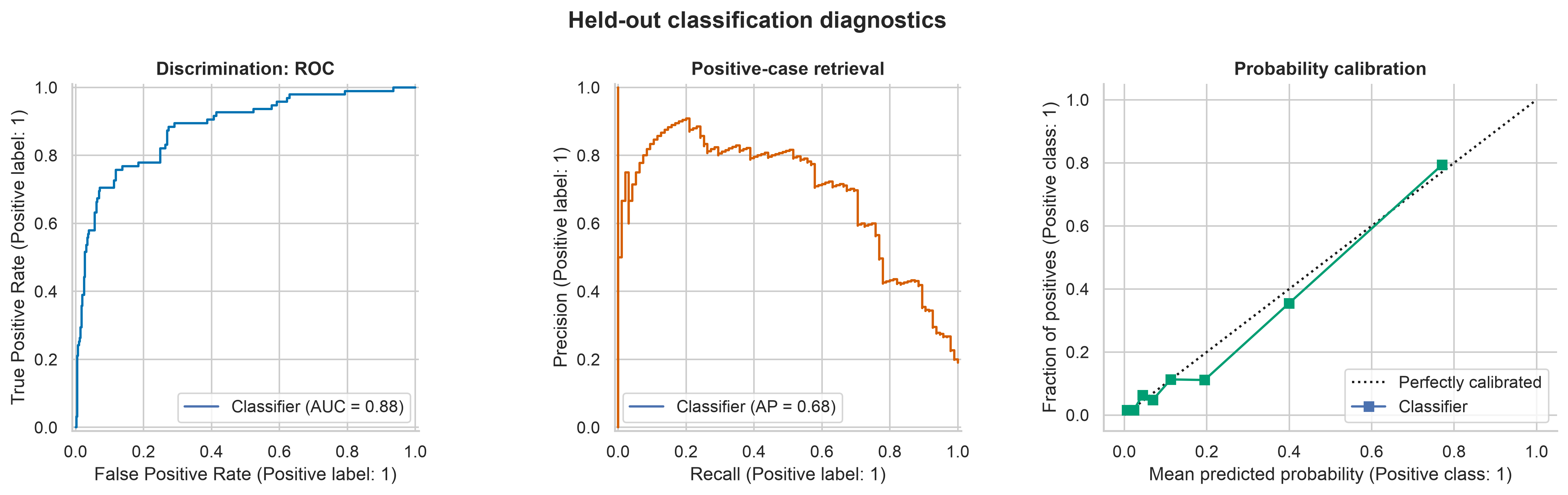
For rare positive outcomes, report precision–recall performance alongside ROC AUC. When probabilities inform decisions, evaluate calibration in addition to discrimination.

from sklearn.metrics import (
    average_precision_score,
    brier_score_loss,
    classification_report,
    log_loss,
    roc_auc_score,
)

test_probability = model.predict_proba(X_test)[:, 1]
test_prediction = (test_probability >= 0.50).astype(int)

print(classification_report(y_test, test_prediction))
print("ROC AUC:", roc_auc_score(y_test, test_probability))
print("Average precision:", average_precision_score(y_test, test_probability))
print("Log loss:", log_loss(y_test, test_probability))
print("Brier score:", brier_score_loss(y_test, test_probability))

Regression metrics

Metric	Interpretation	Important caution
MAE	Mean absolute error in outcome units	Treats errors linearly
RMSE	Square-root mean squared error	Gives greater weight to large errors
Median absolute error	Typical robust absolute error	Can hide large tail errors
\(R^2\)	Improvement over predicting the mean	Does not measure calibration or practical usefulness
MAPE	Mean percentage error	Unstable when observed values are zero or near zero

Always compare the model with a meaningful baseline, such as predicting the training-set mean, median, prevalence, or current operational rule.

from sklearn.dummy import DummyRegressor
from sklearn.metrics import mean_absolute_error, root_mean_squared_error

baseline = DummyRegressor(strategy="median")
baseline.fit(X_train, y_train)

baseline_prediction = baseline.predict(X_test)
model_prediction = model.predict(X_test)

print("Baseline MAE:", mean_absolute_error(y_test, baseline_prediction))
print("Model MAE:", mean_absolute_error(y_test, model_prediction))
print("Model RMSE:", root_mean_squared_error(y_test, model_prediction))

Thresholds are decision choices

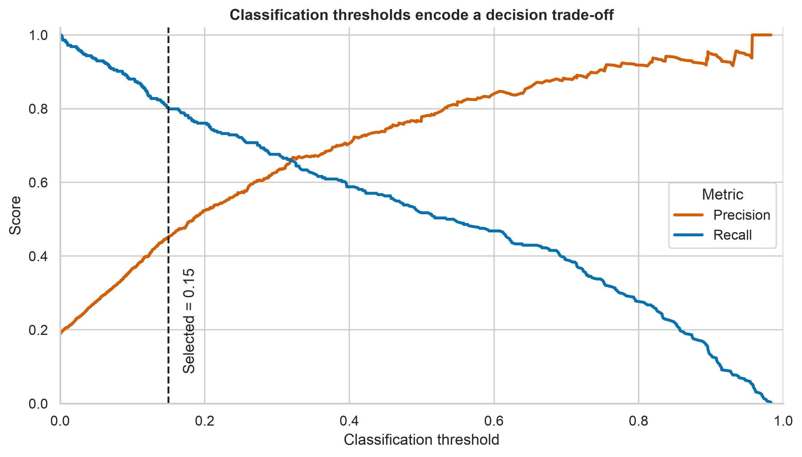
A probability model and a classification decision are not the same object. The default threshold of 0.50 is rarely justified automatically. Select a threshold using validation predictions and an explicit objective, then freeze it before the final test evaluation.

import numpy as np
from sklearn.metrics import precision_recall_curve
from sklearn.model_selection import cross_val_predict

validation_probability = cross_val_predict(
    model,
    X_train,
    y_train,
    cv=cv,
    method="predict_proba",
    n_jobs=-1,
)[:, 1]

precision, recall, thresholds = precision_recall_curve(
    y_train,
    validation_probability,
)

eligible = np.where(recall[:-1] >= 0.80)[0]
selected_threshold = thresholds[eligible[np.argmax(precision[:-1][eligible])]]

This example selects the threshold with the highest precision among candidates that achieve at least 80% recall. A real objective should reflect the costs, benefits, capacity constraints, and ethical implications of decisions.

Discrimination and calibration answer different questions

Discrimination measures whether the model ranks higher-risk cases above lower-risk cases. Calibration measures whether predicted probabilities agree with observed frequencies. A model can discriminate well and still produce unreliable probabilities.

from sklearn.calibration import CalibrationDisplay
from sklearn.metrics import PrecisionRecallDisplay, RocCurveDisplay
import matplotlib.pyplot as plt

fig, axes = plt.subplots(1, 3, figsize=(15, 4.5))

RocCurveDisplay.from_predictions(y_test, test_probability, ax=axes[0])
PrecisionRecallDisplay.from_predictions(y_test, test_probability, ax=axes[1])
CalibrationDisplay.from_predictions(
    y_test,
    test_probability,
    n_bins=8,
    strategy="quantile",
    ax=axes[2],
)

plt.tight_layout()
plt.show()

The project script generates a publication-ready evaluation summary:

python scripts/python/09-generate-model-evaluation-figures.py

Or run the equivalent Bash wrapper:

bash scripts/bash/09-generate-model-evaluation-figures.sh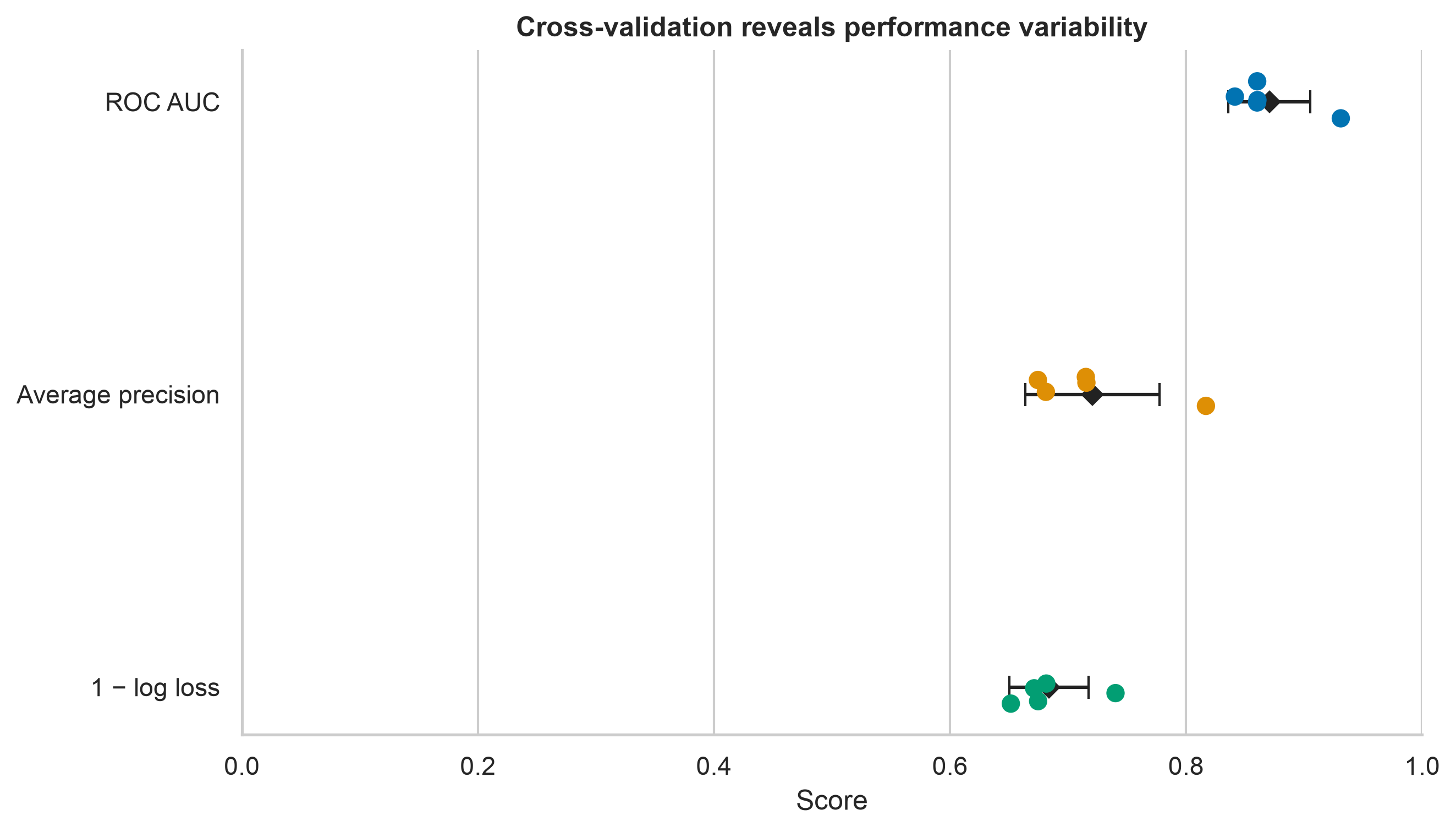

Cross-validated performance across folds.

ROC, precision–recall, and calibration diagnostics on held-out data.

Precision and recall across classification thresholds.

Quantify uncertainty

Test-set metrics are estimates, not constants. Confidence intervals can be obtained with bootstrap resampling when the sampling structure is respected.

import numpy as np
from sklearn.metrics import roc_auc_score

rng = np.random.default_rng(42)
bootstrap_auc = []

for _ in range(2_000):
    index = rng.integers(0, len(y_test), len(y_test))
    sampled_y = np.asarray(y_test)[index]
    sampled_probability = test_probability[index]

    if np.unique(sampled_y).size == 2:
        bootstrap_auc.append(roc_auc_score(sampled_y, sampled_probability))

lower, upper = np.quantile(bootstrap_auc, [0.025, 0.975])
print(f"ROC AUC 95% bootstrap interval: {lower:.3f} to {upper:.3f}")

For clustered data, resample clusters rather than individual rows. When comparing models, apply both models to the same resampled observations so the comparison remains paired.

Examine subgroup performance and robustness

An acceptable overall score can conceal poor performance for an important subgroup. Where sample size and governance permit, examine metrics by relevant groups such as site, region, age band, device, or acquisition period.

evaluation = X_test[["site"]].copy()
evaluation["outcome"] = np.asarray(y_test)
evaluation["probability"] = test_probability

subgroup_auc = (
    evaluation.groupby("site", observed=True)
    .apply(
        lambda data: roc_auc_score(data["outcome"], data["probability"])
        if data["outcome"].nunique() == 2
        else np.nan,
        include_groups=False,
    )
    .rename("roc_auc")
)

Subgroup results require uncertainty intervals and sample counts. They should be interpreted in context rather than reduced to a single fairness claim. Robustness checks may also include missingness patterns, shifted prevalence, measurement changes, and performance over time.

A reproducible evaluation workflow

Use the following sequence to protect the final estimate:

1. Define the prediction target, unit of observation, intended use, and error costs.
2. Choose a split that represents the deployment scenario.
3. Reserve the test set before exploratory model comparison.
4. Place all learned preprocessing and feature selection inside a pipeline.
5. Establish a simple baseline.
6. Tune models and thresholds using training data and validation procedures only.
7. Inspect fold variability, discrimination, calibration, and relevant subgroups.
8. Freeze the complete workflow, metric set, and threshold.
9. Evaluate once on the test set and report uncertainty.
10. Plan external or prospective validation and post-deployment monitoring.

What to report

A transparent model evaluation report should include:

• dataset source, eligibility criteria, sample size, and outcome prevalence;
• unit of splitting and any grouping or temporal constraints;
• preprocessing, feature selection, model, and hyperparameter search space;
• validation design, number of folds or repeats, and random seed;
• baseline and primary metric selected before final evaluation;
• secondary metrics, threshold rule, calibration, and subgroup analyses;
• point estimates with uncertainty intervals;
• missing-data handling and leakage controls;
• intended population and known limitations; and
• conditions requiring recalibration, retraining, or model retirement.

Common mistakes

Mistake	Why it is misleading	Better practice
Reporting training performance	Measures fit to seen data	Use validation and held-out test data
Preprocessing the complete dataset	Leaks validation information	Fit preprocessing inside each training fold
Optimizing many models on one test set	Turns the test set into validation data	Keep one untouched final test set
Reporting only accuracy	Conceals error types and imbalance	Report task-relevant threshold and probability metrics
Selecting 0.50 automatically	Ignores decision costs	Tune the threshold on validation predictions
Reporting only mean CV performance	Hides instability	Show fold scores or uncertainty
Treating internal validation as universal proof	Ignores distribution shift	Validate across time, sites, or external data

Chapter summary

Reliable evaluation is a design problem, not a final calculation. The split must represent intended use, preprocessing must remain inside the validation loop, metrics must reflect the consequences of error, and the test set must be protected from model selection. Strong validation combines discrimination, calibration, uncertainty, subgroup assessment, and transparent reporting.

The next chapter can build on this evaluation framework by moving from internal performance estimates to model interpretation, deployment readiness, or monitoring—depending on the guide sequence.